Blog post for paper "Rethinking Fine-Tuning when Scaling Test-Time Compute"
Direct Coverage Optimization: first an analogy
Before diving into specific results from the paper (here is the link for convenience) we will start with an analogy. We call our analogy the Multiversal Stochastic Bookie Horse Race Problem. Quite a mouthful. Hopefully that will make more sense in a bit.
Imagine you are betting on a horse race, but in pretty unusual circumstances. Namely, you place a bet with a bookie that acts stochastically, all you can ask for is a set of probabilities across outcomes. Then the bookie and a set of additional N-1 of his multiversal copies place the bets, each independently. When the horse race is run, you get rewarded if the horse that won had at least one of the multiversal bookies place a bet on them. You get rewarded no more or no less if the winning horse had more than one bookie place a bet on them. A bit strange, we know. Let’s start with a two horse race. Let’s say that one horse is more likely to win than the other and you have a bookie that bets on that horse with probability $p_1$. Assuming that horse one indeed wins, what is your probability of being rewarded as function of the bookie’s probability to place a bet on horse one? It is more easily expressed through its complement. The only way you lose is if in all $N$ universes the bookie placed a bet on the other horse. Since there are only two horses, the probability of placing a bet on the other horse is just $(1-p_1)$. Therefore the probability of the other horse being picked is $(1-p_1)^N$. The probability of winning is the complement of that: $1 - (1-p_1)^N$.
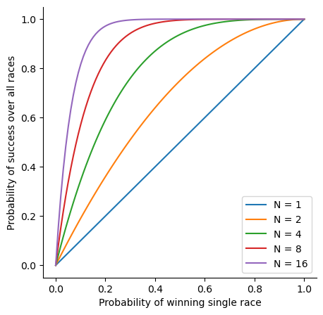
Here is a plot of your chance of winning the multiversal horse race as a function of $p_1$ for three values of $N$. More precisely this is a plot of your chance of winning assuming horse one indeed won. We will assume that is true for the next couple of parts for simplicity, then revisit it considering the chance that horse actually did win.

Nothing surprising here. For a fixed $N$ your chances of winning are larger for larger $p_1$ and for fixed $p_1$ are larger for larger $N$.
Let’s move to a slightly more complicated situation. The horse race now has k horses. For simplicity we will look only at the probabilities of the bookie placing a bet on two horses: $p_1$ and $p_2$. Note that since there are many horses these probabilities no longer need to sum to 1. Now imagine that we just bet on a race where the bookie worked with probabilities (…, 0.1, 0.2). The master of the multiverse (what is the name of the big bald guy with the cape?) asks us whether we would like to switch to a different bookie that has probabilities: (…. 0.05, 0.5). Should we take it? Intuitively we would say of course we should. We increased the chance of putting a bet on the horse most likely to win by a large fraction and we reduced the probability of the next likeliest by a small fraction. This intuition is correct for N=1. However the surprising thing is that it is not correct for high N.

What do we mean by that? Well, in brief our intuition is used to thinking of maximizing winning a single bet, or to a related situation in which we want to maximize the number of times we got the bet right (and that is also the scenario many classic optimization portfolio problems deal with). But that is simply not the setup here. We are rewarded for placing the correct bet at least, and no more if we get it right multiple times. Figure 2 helps us think through that. All three subpanels show the probability off winning a single race on the x-axis and the overall probability of success on the y-axis. The original offer is in blue. The second offer is in red. Each offer is plotted twice. Once for $N=1$ and once for $N=16$. Start from the leftmost subpanel. Let’s compare points first for $N=1$, i.e., the points sitting on the blue curve. This is the part that follows our intuition. We raised the probability of the most likely horse (the slightly larger scatter point). Accordingly the x and y values of the larger point increased. We lowered the probability of the second-most-likely horse. Accordingly the x and y values decreased. The middle panel has little i-beam lines to help us see the increase in success probability between the original and second offer. The more probable horse increased by a lot and the second-most-likely horse decreased by a little. The rightmost panel shows us however what happens for a moderately high $N$, $N=16$. Due to the non-linearity of the relation between the probability of winning a single race and the probability of winning at least one race, the original offer was already almost guaranteed to have at least one bet on the most probable horse, i.e., the larger blue dot is close to a value of one. While this probability did increase as it has to with increasing the probability of a bet in a single race, the increase was very small (it is a little hard to even see the i-beam in the plot). In contrast, the small reduction in the probability of the second-most-likely horse in an individual bet turned into a large decrease in the probability of overall success, again due to the non-linearity of the curve.
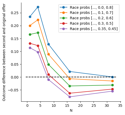
But does it matter that we reduced the probability of a horse that is less likely to win? Isn’t it still worth it since we did increase the probability of the horse most likely to win, even if it is by a little bit? Well, it depends how likely is the horse most likely to win to indeed win and how that compares to the second-most-likely to win. Up until now we ignored the actual outcome of the race and just considered the outcome of the stochastic betting process itself. If we introduce some values for the probability of the outcome of the actual race we can close the loop and actually say whether we should accept the offered change of bookie or not. The following plot gives a sense of that:

As can be seen, for $N=1$ our intuition is correct: no matter what the underlying probabilities (different curves) might be, we should accept the offer (y-axis value greater than zero). However, as N increases the situation reverses and almost always we shouldn’t accept the change in offer (y-axis value lower than zero), despite how appealing it might look with the large increase in the probability of placing a bet on the most likely outcome. This is because the nonlinear transformation from single race bet placing probability to at least one race bet racing probability makes the increase of the at least one race probability of the most probable outcome small and the decrease of the second-most-probable large.
Back to LLMs
At this point we have probably belabored the story too much and the analogy is clear. The bookie is the LLM. It is stochastic since output generation in LLMs is typically stochastic. The N universes are the N times that we are allowed to call the LLM. The strange betting reward scheme is a translation of the class of problems that we discuss in the paper, i.e., problems in which we are asked to obtain a correct answer with $N$ tries and there are no positive consequences (no “extra credit”) for multiple correct answers unlike more traditional portfolio betting problems.
In the context of LLMs we of course don’t get to pick a specific bookie, rather we train the LLM (or to be more precise here in academia we fine tune the LLM). This changes the weights of the networks which changes the probabilities of generating different responses, which is the analogy to choosing different bookies. However, we can still think of training as a choice between an original bookie (the non finetuned model, or a model finetuned to some degree) to a different bookie (a more finetuned model). We do choose whether to finetune, how much to finetune and based on which datasets. Just as the discussion of the multiversal stochastic bookie horse race problem clarifies (hopefully), we can’t naïvely assume that offers that seem like a good idea for $N=1$ will work for higher $N$. Rather, since we know what we want to maximize, coverage at some $N$, then we need to optimize for that and not some other more traditional, intuitive error function.
Finally back to the paper
In the paper we directly derive a loss function specific to the pass@N objective. We refer to it as the Direct Coverage Optimization (DCO) since it directly optimizes for coverage. The difference of this loss is most easily appreciated through its gradient which is (slightly simplified from the paper): \begin{equation} % \nabla_\theta \ell_{\text{DCO}}^N(x,y) = F\left(N,\hat{p}(y|x)\right) \nabla_\theta \ell_{\text{CE}}(x,y) \nabla_\theta \ell_{\text{DCO}}^N = F\left(N,\hat{p}\right) \nabla_\theta \ell_{\text{CE}} \label{eq:DCO-gradients} \end{equation} where $\ell_\mathrm{CE}$ is the standard cross entropy loss, $\hat{p}$ reflects the models current distribution of outputs (the analogy of the probability of a bookie placing bets with varying probability on different horses). $F(N,\hat{p})$ is an extra factor that appears in the derivation and multiplies the standard cross entropy gradient. This means that there is a specific, different loss function we should use if we want to optimize for pass@N. This factor $F$ is given by: \begin{equation} F(N,\hat{p})=\frac{N (1-\hat{p})^{N-1}\hat{p}}{1-(1-\hat{p})^N} \label{eq:DCO-gradients-factor} \end{equation} If you work through the expression for a bit you can convince yourself that this factor is equal to one for $N=1$ meaning that our gradient becomes the regular cross entropy gradient for $N=1$.
We then show empirically that the concerns raised by the multiversal stochastic bookie horse race problem indeed arise in real applications. Table 1 of our paper, reproduced here, shows that when finetuning for mathematical reasoning, performance of pass@N actually decreases over training epochs with regular cross entropy loss, just as the seemingly very promising offer to switch a bookie in the example above actually reduces overall outcome at high N.
| pass@1 | pass@16 | pass@256 | pass@4k | |
|---|---|---|---|---|
| Epoch 1 | 4.4% | 30.0% | 65.2% | 82.5% |
| Epoch 2 | 5.3% | 31.4% | 64.5% | 80.0% |
| Epoch 3 | 6.5% | 28.7% | 54.5% | 79.2% |
| Epoch 4 | 7.4% | 22.9% | 44.5% | 63.0% |
Table 1: Pass@N coverage results on the MATH test set for a Llama-3-8B-base model fine-tuned with cross entropy loss on direct answers from the MATH training set. Pass@N test accuracy at large $N$ decreases with number of training epochs, just as in the concern with replacing current bookie with bookies that over favor the most likely option
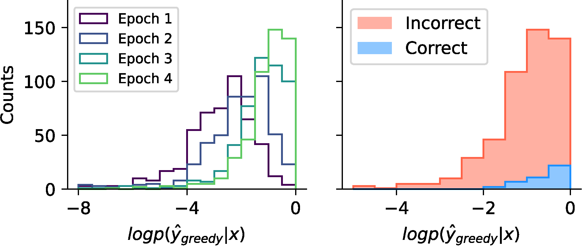
Next we tie together the empirically worse performance we observe and the notion of picking a bookie that is good at placing bets on the most probable horse but at the cost of other horses. In Figure 4 (part of Figure 1 in the paper) we show that with cross entropy loss, the probability of assigning an output to the most likely completion grows over training, akin to accepting offers to trade bookies that have larger probability of placing a bet on the most probable horse, despite the possible unfavorable tradeoff. Furthermore, we show that sometimes this completion is even wrong, which is more problematic still. In the paper we also show that with our loss function this potential over increase in confidence is ameliorated.

What else? In figure 3 above we just picked specific probability values and plotted the resultant curves. As one might guess, given that we know the functions involved in calculating outcomes, we can make more precise statements about tradeoffs and what type of “bookies” are most favorable. We prove two lemmas with bounds on the confidence (our bookie probability) of the most likely outcome.
Finally, we consider a more complex case arising in Chain of Thought (CoT) reasoning. The key difference is that though there is still a correct answer to a query, there are numerous possible intermediate outputs that we are neutral to. For instance, we don’t mind if the chain of thought starts with: “Let’s see, I think the answer is:…” Or “Thinking step-by-step I first tried… finally I see the answer is:…” or any of many other variants. Adapting to this regime required non-trivial engineering. Briefly put, we showed that the same issues we discuss above are relevant for CoT and our loss function improves results though the gaps were smaller.
There is more detail in the paper, but hopefully this serves as a good start to get the gist of it.